Path Planning
Computational Geometry
How to represent object in 1D, 2D, and 3D?
1D: Lines, Curves
- Points/Line segments: Just explode the path into a bunch of points, implicitly connected by line segments. Despite the simplicity, with enough points you can approximate any curve to arbitrary accuracy.
- Line segments and Other Primitives: We can add add some other primitives to our line segments. Arcs are the most common addition. In G-Code G01 is a straight line, G02 is a clockwise arc, and G03 is a counter-clockwise arc. G-Code Viewer is a great way to visualize G-Code.
- Spline: There are a lot of different splines, which ultimately are all ways to parametrize curves with different forms of polynomials (or ratios of polynomials). Splines are named after the wooden tools that were used by architects and boat builders (among others) to repeatably draws curves before all these newfangled computers. Cool videos about Splins if you want to learn more:
-
Implicit curve:
a plane curve defined by an implicit equation relating two coordinate variables,
commonly x and y.
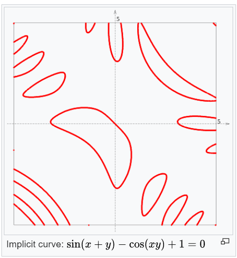
- Discretized Points: We can use simple line segments, but constrain the points to lie on the vertices of some lattice. As we will see, doing so can drastically change the nature of the relevant path planning algoritms, since we will be solving discrete problems instead of using floating point numbers to approximate real numbers.
2D
- Meshes: Connecting points with sections of planes to form 2D surfaces. Often meshes are restricted to use triangles, but you may also see quad, hex, or mixed meshes.
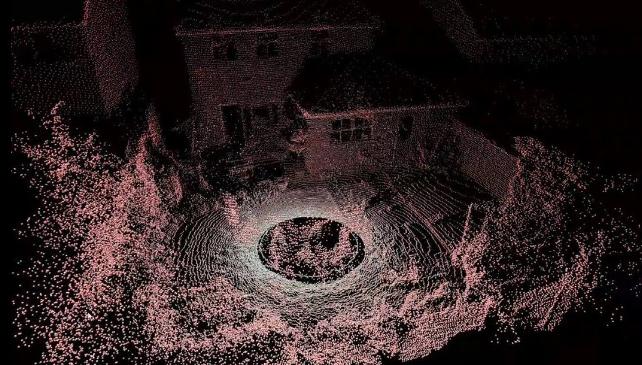
- Point Clouds: If we take a mesh and throw away the connectivity information (which points should be connected to form triangles), we just left with the points. Sometimes this is all we need. Other times, it all we get, as with many 3D scanning techniques.
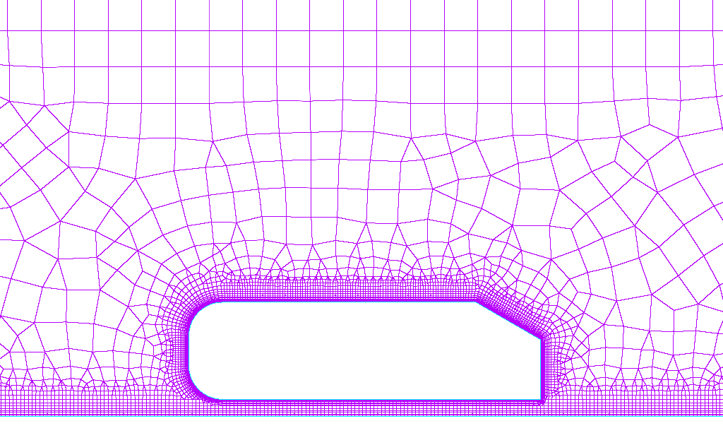
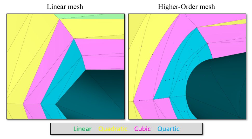
- High Order Mesh: connects adjacent mesh points with a curve of polynomial degree higher than one (i.e. linear). The easiest way to understand high-order meshing is to compare a high-order mesh with a linear mesh. In a linear mesh, volume cells are constructed from a set of straight lines connecting grid points. A high-order mesh connects grid points with a non-linear polynomial function (e.g. second degree quadratic), thus the technique is called "mesh curving."
- Fixed Point Meshes: We can constrain the points used to define our mesh to lie on the vertices of a lattice.
- Other Primitives: Just as we combined arcs with line segments in 2D, we can add sections of surfaces like cylinders and cones to the planar sections commonly seen in meshes. The boundaries between primitives necessarily end up being more complex than in meshes, since cylinders and cones are not planar.
- Implicit Surfaces The level sets of an algebraic expression involving x, y, and z (or some other three dimensional coordinate system) are 2D surfaces.
- Splines: Splines work just as well for 2D objects as they do for curves. All of the splines we have seen so far can be generalized to 2D. NURBS (Non-uniform rational B-spline)
3D
- Meshes We can keep generalizing the “connect points with linear elements” strategy. To represent a volume, we just use meshes of 3D objects like tetrahedra instead of 2D objects like triangles (or 1D objects like line segments).
- Fixed Point Meshes: We can constrain the points used to define our mesh to lie on the vertices of a lattice.
- Point Clouds: We can also just sample a bunch of points from within a volume. Among other things, this is useful for seeding particle based simulations.
- Boundary Representations (B-reps): any closed surface defines a volume. So we can use any of the above 2D representations to represent 3D shapes as well. Most common CAD programs use B-reps based on geometric primitives like planes and cylinders, augmented with splines and meshes.
- Splines: We can use splines with three parameters to directly describe volumes. NURBS (Non-uniform rational B-spline)
- Implicit Volumes (F-reps): We can represent volumes directly with algebraic expressions of x, y, and z (or other three dimensional coordinate systems). Instead of taking level sets, we consider regions where the expression is above (or below) some threshold (usually zero). A particular case is signed distance fields, in which the value at each point represents the distance from that point to the boundary of the volume, with negative values given for internal points.
- Voxels: If we discretize our space, usually into tiny cubes, then we can just specify which elements are in the shape and which are not. This is arguably the simplest representation format to describe and process, but it can end up being extremely memory intensive. As a result, various approaches exist to compress voxel data, usually using hierarchical data structures like octrees. Flocks of assembler robots show potential for making larger structures
- Adaptively Sampled Distance Fields: This is a combination of signed distance fields and voxels (or pixels, if we do the same thing in 2D). The basic idea is to sample a signed distance field in the center of each voxel. To make it adaptive, we use an octree or some other hierarchical structure to compress the data, allowing the resolution to change as needed across the volume.

Control
- Point to point: move from one point to another without following the line between the two pints.
- Point to point along a line path: involves acc calculation, not violate the max acc.
- Along a path: corners operations. Basically pretend that you *can* have an infinite acceleration (as long as the actual speed change is small) and let the physics of the real world act as your low pass filter to smooth things out. So at each vertex, you compute the speed change for each axis. If it's below a threshold (which motion planners often call the "jerk") then you apply the speed change instantaneously in the motion planner.
- Output control pulses: update distance and output pulse if the distance hit a step trigger.
2. Subtractive process
a. 2D
How does Mods milling PCB work?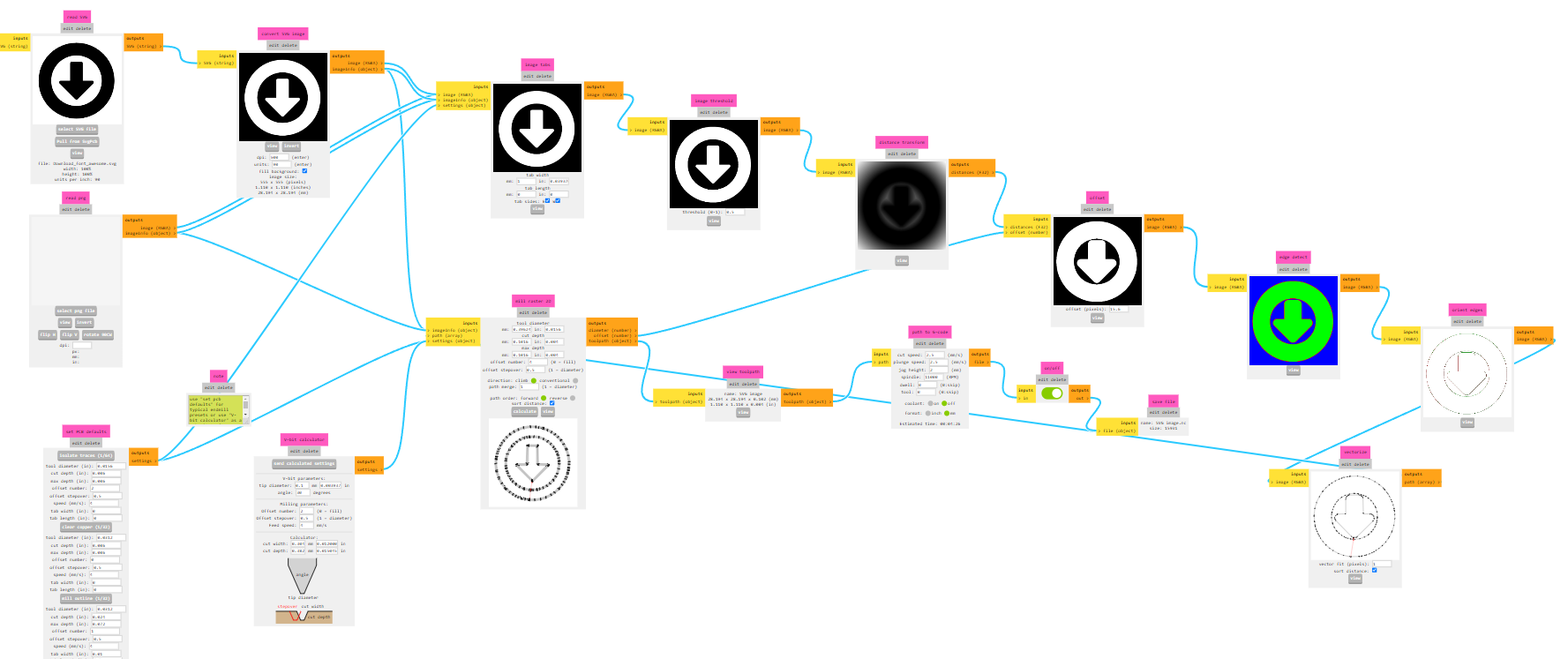
- resize image and threshold input image to binary image.
- distance transform
- Euclidean Distance Transform (EDT): iterate all foreground pixels with the all background pixels (high computational cost) calculating the square value is better, this still includes square calculation, and float data operations.
- Chamfer Distance Transform: use a weight matrix to iterate all pixels, and update the distance value based on current distance value (chamfer_distance_transform.py).
- Manhattan Distance Transform (MDT): distance is the absolute difference between the pixel and the nearest background pixel. (Manhattan_Distance_Transform.py)
- Chebyshev Distance Transform (Chessboard Distance, CDT): the maximum difference along any axis (X or Y). (Chebyshev_Distance_Transform.py)
- What Mods uses : Chebyshev Distance Transform: the minimum difference along any axis (X or Y). add image here, right/left/top/down scan.
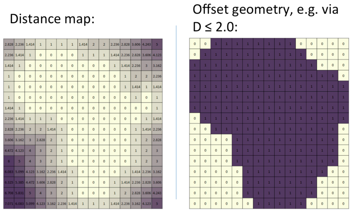
- Offset based on tool configuration.
- Edge detection.
- Orient edges.
- Vectorize edges.
Use RGB value to threshold the image. R+G+B/(3*255)
Use distance transform to get the distance from the edge of the image.
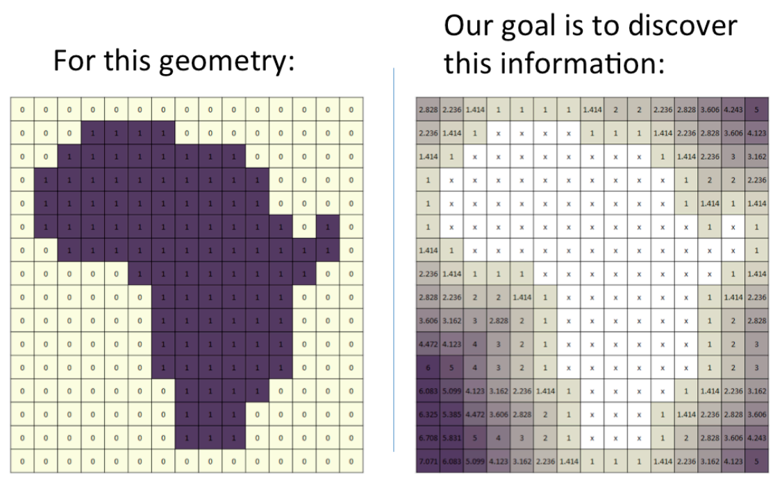
Off-the-shelf functions: OpenCV scipy
Offset the boundary based on the tool diameter, Offset setting (binary to RGB-alpha data).
Scan all pixels within a 3x3 grid.
Check each edge section's orientation based on the relationship with adjacent edge pixel.
Start from one edge pixel, Vectorize all edges based on the orientation of the edge from the last step.
b. 3D
- Zig-zag: For facing large areas with no potential collisions, you can just go back and forth across the whole surface. The separation between adjacent lines is determined by your step-over.
- Spiral: Another strategy is to use a spiral instead of a zig zag path.
- Offset: Area with walls that we can not crash into. Offset paths are also what are used to finish vertical walls (with a side or swarf milling cut).
- Swarf Toolpath: This is an offset path for a (developable) surface, Offsets of planar, conical, and cylindrical faces can be determined analytically.
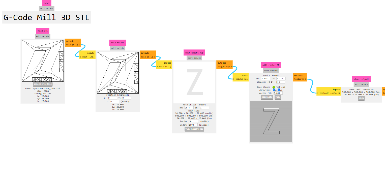
- Read STL and rotate as needed
- Map height: find the limits of the mesh, analyzing the vertices of each triangle in the mesh data.
- Generate toolpath: It iterates over the height map, constructing the tool offset and determining the toolpath based on specified directions. It iterates over each point in the height map, moving the tool along the surface while considering the tool offset. The algorithm follows the surface, adjusting the tool position based on the stepover and error tolerance.
c. Fast machining path planning
- Challenges: lower the tool vibration (tool breakage, poor surface finishing, needs some damping mechanism) (IMU) ; more tool service life (accelerate tool wear); heat generation; Material Compatibility (very hard material).
- Generating optimized toolpaths that maintain constant chip load, minimize tool engagement, and reduce sudden directional changes can enhance machining efficiency and surface quality.
- Research trends in high speed milling of metal alloys: A short review Omag Tower 7 - Seven Axis CNC Work Center